Create 3D composition space plots

The same packages are required as in the 2D plots notebook:

import matplotlib.pyplot as plt
import compspace as cs
import pandas as pd
import numpy as np

Load the sample example data file as well:

# Load example data
comps = pd.read_csv('comp_example.csv', index_col=0)

# Function to create a subset of given constituents
def create_subset(c: pd.DataFrame, constituents: list[str]) -> pd.DataFrame:
    # Create the subset with the given constituents and re-normalize to 100 at.%
    subset = c[constituents]
    return subset.div(subset.sum(axis=1), axis=0) * 100

# Visualize the DataFrame
comps.head()

	Cr	Co	Cu	Fe	Mo	Mn	Ni	Ti
Index
1	15.28	4.13	18.34	33.47	6.52	4.84	10.10	7.32
2	15.53	5.10	18.63	33.31	8.60	3.75	8.73	6.35
3	14.24	5.64	17.09	32.04	9.55	6.15	8.91	6.37
4	12.70	6.56	15.24	32.01	11.33	6.75	9.41	6.01
5	12.65	6.22	15.18	33.19	11.24	6.79	8.15	6.59

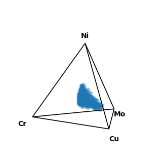
Currently, only quaternary (4-component) and quinary (5-component) composition spaces are supported for 3D plotting. Instead of compspace2D the projection compspace3D is needed for the 3D plots. The rest of the plotting functions are similar to the 2D case, however, there are no ticks and grids. Here is an example for a quaternary composition space, which plots a tetrahedron in 3D:

# Create a quaternary subset
quaternary_subset = create_subset(comps, ['Cr', 'Cu', 'Mo', 'Ni'])

# Create a figure with a quaternary projection, but now in 3D
fig, ax = plt.subplots(figsize=(4, 4), subplot_kw={'projection': 'compspace3D'})
# Scatter the data points
sc = ax.scatter(quaternary_subset, alpha=0.3)
# Show the plot
plt.show()

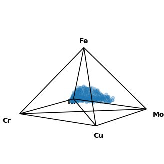
If you are running this on your on machine, you can make use of the interactive plotting capabilities of matplotlib by adding %matplotlib qt to the beginning of a jupyter notebook cell. This opens the plot in a separate interactive window. For more than four constituents, three dimensions are no longer sufficient to represent the full composition space. Therefore, for quinary and higher, the dimensionality needs to be reduced. In this package, this is done by plotting a pyramid with a rectangular base. This has the disadvantage that the distances between the individual vertices is not always identical, which needs to be kept in mind when interpreting the plots. Here is an example for a quinary composition space:

# Create a quinary subset
quinary_subset = create_subset(comps, ['Cr', 'Cu', 'Mo', 'Ni', 'Fe'])

# Create a figure with a quaternary projection, but now in 3D
fig, ax = plt.subplots(figsize=(4, 4), subplot_kw={'projection': 'compspace3D'})
# Scatter the data points
sc = ax.scatter(quinary_subset, alpha=0.3)
# Show the plot
plt.show()

Animation

compspace also supports the creation of rotation animations for the 3D composition space plots. For this, there is an additional function rot_animation(...) which takes the figure and axis objects as input. Also, the number of frames and the resolution can be specified. To ensure the animation is created properly, make sure ffmpeg is installed on your system. The python version of that is automatically installed when installing the compspace package, but the base version needs to be installed manually from here. The creation of the animation will still work without it, but matplotlib will fall back to pillow which can have some side effects.

# Create a quinary subset
quinary_subset = create_subset(comps, ['Cr', 'Cu', 'Mo', 'Ni', 'Fe'])

# Create a figure with a quaternary projection, but now in 3D
fig, ax = plt.subplots(figsize=(4, 4), subplot_kw={'projection': 'compspace3D'})
# Scatter the data points
sc = ax.scatter(quinary_subset, alpha=0.3)
# Animate the plot
#cs.rot_animation(fig, ax, path='rot_animation.gif')  # comment in if you execute this on your own machine
# Show the plot
plt.show()