Convenience function

If you just want to quickly plot compositions on a composition space without worrying too much about the plotting details, you can use the convenience function. It allows to plot compositions on a 2D or 3D composition space with minimal code. First, import the package to access the function.

import compspace as cs
import pandas as pd

Load the example data from a .csv with pandas. We also define a function to create subsets of the constituents. The dataset is a simulated materials library of an 8-component alloy system with 342 individual compositions.

# Load example data
comps = pd.read_csv('comp_example.csv', index_col=0)

# Function to create a subset of given constituents
def create_subset(c: pd.DataFrame, constituents: list[str]) -> pd.DataFrame:
    # Create the subset with the given constituents and re-normalize to 100 at.%
    subset = c[constituents]
    return subset.div(subset.sum(axis=1), axis=0) * 100

# Visualize the DataFrame
comps.head()

	Cr	Co	Cu	Fe	Mo	Mn	Ni	Ti
Index
1	15.28	4.13	18.34	33.47	6.52	4.84	10.10	7.32
2	15.53	5.10	18.63	33.31	8.60	3.75	8.73	6.35
3	14.24	5.64	17.09	32.04	9.55	6.15	8.91	6.37
4	12.70	6.56	15.24	32.01	11.33	6.75	9.41	6.01
5	12.65	6.22	15.18	33.19	11.24	6.79	8.15	6.59

The convenience function takes a DataFrame or a list of DataFrames, automatically decides whether to plot in 2D or 3D, creates a matplotlib figure and plots the compositions as a scatter plot. The function also accepts a variety of the standard scatter keyword arguments to customize the plot, however, if you want full control, you should visit the other guides for more customization options.

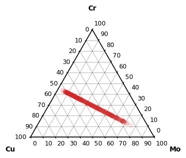
# Create a ternary subset
ternary_subset = create_subset(comps, ['Cr', 'Cu', 'Mo'])

# Call the convenience function
cs.plot_on_comp_space(ternary_subset, alpha=0.1, c='tab:red')

(<Figure size 400x400 with 1 Axes>, <CompSpace2DAxes: >)

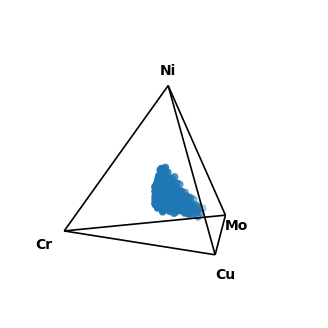
The convenience function will default to 3D plots whenever possible to avoid condensing too much information into 2D. Here, we create a quaternary subset and the function automatically creates a 3D plot.

# Create a quaternary subset
quaternary_subset = create_subset(comps, ['Cr', 'Cu', 'Mo', 'Ni'])

# Call the convenience function again
cs.plot_on_comp_space(quaternary_subset)

(<Figure size 400x400 with 1 Axes>, <CompSpace3DAxes: >)

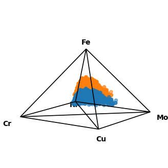
It is also possible to plot multiple subsets at once by passing a list of DataFrames. Here, we create two quinary subsets and plot them together in one pyramid plot. Be aware that this only makes sense if all subsets have the same constituents.

# Create a quinary subset
quinary_subset_1 = create_subset(comps, ['Cr', 'Cu', 'Mo', 'Ni', 'Fe'])
# Artificially increase the Fe content and re-normalize
quinary_subset_2 =  quinary_subset_1.copy()
quinary_subset_2['Fe'] = quinary_subset_2['Fe'] * 2
quinary_subset_2 = quinary_subset_2.div(quinary_subset_2.sum(axis=1), axis=0) * 100

# Plot both subsets into the same composition space
cs.plot_on_comp_space([quinary_subset_1, quinary_subset_2])

(<Figure size 400x400 with 1 Axes>, <CompSpace3DAxes: >)

The convenience function returns the created matplotlib figure and axes, which allows for further customization of the plot fig, ax = cs.plot_on_comp_space(...).